What Axiom Border is

Most edge monitoring works one way: a collector gathers data, ships it somewhere, and a platform decides what it means. Take the link away and the collector is a data recorder at best.

Axiom Border is built on the opposite premise. It is not an agent that reports to a cloud. It is an autonomous node that observes the network around it, decides what matters against rules it holds locally, and acts on that decision — on the machine, with no server in the loop. Centralising into OpenGate is something you switch on afterwards if a fleet-wide view is useful to you. It is never what makes the probe work.

That single decision is why the product looks the way it does:

• The decision engine is on the probe. Alarms are raised where the data is, not where the platform is.
• Everything it needs travels with it. The vulnerability database, the vendor registry, the MIB catalogue, the scan templates, the metrics store, the container runtime and the web console are all installed with the product. A probe in an isolated network is useful the moment it starts.
• Nothing is fetched at run time. There is no feed to update before a scan means anything, and no service to call before a finding can be interpreted. What exactly it carries, where each data set comes from and how to refresh it in the field is set out in Catalogs: vulnerabilities, OIDs, MIBs and more.

Why this matters in an industrial network

Isolated OT segments are isolated on purpose. A tool that needs to reach the internet to stay useful is a tool that is either useless there or a hole in the isolation. Axiom Border needs neither.

The specification, in one table

Deployment roles	central — the full node: probe, metrics store and the container runtime for the AI capability. monitoring — a remote node that reports into a central one
Installation path	A single supported path, the Keystone deployment agent, and it is 100 % offline. Roughly 5–8 minutes for a central node, 1–2 for a monitoring one
Footprint	About 141 MB for a central core package and 89 MB for a monitoring one, plus the bundled data packs, which are published once and reused across versions
Management surface	The embedded web console and a REST API, both served by the probe itself, both over HTTPS unconditionally — localhost included
Internet access	Not required, at install time or afterwards

HTTPS is not optional

There is no plaintext listener to fall back to. A probe reached over http:// refuses the connection, and that applies to localhost as much as to anything else. On first boot the probe issues its own certificate from a local authority, so it works with no PKI and no internet — see Security posture for replacing it with your own.

The two roles

A single probe covers a site on its own. The roles exist for when one site is not the whole picture.

flowchart LR
    M1["monitoring<br><i>remote node</i>"] --> C
    M2["monitoring<br><i>remote node</i>"] --> C["<b>central</b><br>probe · metrics store<br>console · AI"]
    C -.->|optional| OG["OpenGate"]:::ext
    classDef ext fill:#e9edfa,stroke:#486ac9,color:#101010

A central node is a complete Axiom Border: it watches its own network, holds the history, serves the console, and can additionally receive from monitoring nodes. A monitoring node is the light end of the fleet — it watches the machine it runs on and reports into the central one.

The dotted arrow is the point. OpenGate sits outside the boundary, it is optional, and it starts switched off.

How you work with it

Through the console. The probe serves its own web interface; point a browser at its address and log in. Everything on the pages that follow is described from that interface, because that is how the probe is meant to be operated.

A REST API exists underneath for integrating the probe with your own systems, and OpenGate drives the probe over it. It is not the operator’s path.

The console has six views, in the order the sidebar lists them:

View	What it is for	Where it is documented
Network status	Everything discovered on the network: assets, ports, vulnerabilities, and the passive inventory behind them	Security assessment
Hosts Status	The machines running a monitoring agent, one block per node	Metrics and monitoring
Alerts	Raised alarms, alarm history, and the rules behind them	Alarms and rules
Supervisions	The monitoring agents reporting in and what each last delivered	Metrics and monitoring
AI capabilities	Anomaly-detection models running on the probe	AI capabilities
Configuration	The probe’s own settings, edited and applied from the browser	Configuration

Network status is the landing view, which tells you where the product thinks the centre of gravity is: what is out there, and is it exposed.

Next: The full loop — the four stages a single observation travels through.

Ingest, observe, decide, act

Everything Axiom Border does fits into four stages. They run in parallel and on their own clocks — the numbering follows a single observation through the product, not an order of execution. What binds them together is that all four write to the same local state, and all four can raise an alarm.

flowchart LR
    I["<b>1 · INGEST</b><br>from the machines"] --> O["<b>2 · OBSERVE</b><br>from the network"]
    O --> D["<b>3 · DECIDE</b><br>local rules"]
    D --> A["<b>4 · ACT</b><br>alarm and notice"]
    A -.->|optional| C["OpenGate"]:::ext
    classDef ext fill:#e9edfa,stroke:#486ac9,color:#101010

1 · Ingest — what the machines report about themselves

Every monitored machine runs a lightweight agent that watches it from the inside and sends what it sees. Four monitors, each answering one question:

Monitor	What it watches
SSH-Guard	Interactive sessions and login attempts against the machine
USB-Guard	Devices attached to and removed from its ports
IFACES-Guard	The state of its physical network interfaces
METRIC-Guard	The machine’s own health, and the heartbeat that proves it is still reporting

You see this stage in two views. Supervisions lists the agents reporting in, one card per monitor, with the last event each delivered. Hosts Status turns the same data around and shows one block per machine, with the alarms currently open against it.

2 · Observe — what the probe works out for itself

Four probes on the network, one listening and three asking, each with its own scheduler. This is the stage that needs no cooperation from the equipment it watches, and it is covered in full on the next page: The four probes.

Everything they find lands in Network status.

3 · Decide — rules that run on the probe

Two mechanisms, both evaluated locally against data the probe already holds:

• Rules on each event, as it arrives. One rule set per probe, so a rule can react to a new host, a newly opened port or a changed value the moment it is observed.
• Periodic checks against the history. Counting occurrences over a window, and detecting the absence of them — a node that stopped reporting is a condition you can only see by looking for silence.

Both are edited from Alerts → Rules configuration. Neither needs the uplink, which is the whole point: a probe whose link is down still decides.

4 · Act — the alarm, and who hears about it

A raised condition becomes a coalesced alarm — one alarm with a count, not one alarm per occurrence — which lands on the operator’s Alerts view and in the probe’s live feed, so the console’s counter moves immediately. From event to alarm covers how that works and why it is built that way.

And then, only if you asked for it, the same alarm goes out to OpenGate.

Nothing leaves the machine by default

This is the commercially important half of the loop, so it is worth stating plainly:

• The OpenGate integration is optional and starts inert. It has to be configured and enabled before a single byte goes anywhere.
• The message broker the console listens on lives on loopback. It is not exposed to the network.
• All four probes write to local storage before any decision to publish exists.

A probe you install and never configure for the cloud is a probe that never talks to one. What travels when you do enable it is the complete inventory of your network, which is exactly why the probe refuses to start that integration over an insecure address — see Security posture.

Next: The four probes — the observation stage in detail.

One listens, three ask

Axiom Border looks at the network with four probes. The split that matters is not what they scan but whether they speak: one of them observes without emitting a single packet, and three of them ask questions and read the answers.

Probe	How it works	What it produces	When it runs
Passive analysis	Listens to the traffic reaching its capture interface. Emits nothing	Assets indexed by MAC address, which address belongs to which device, LLDP neighbours, the services actually in use, industrial protocols in play, traffic volume per host, what kind of point the probe is plugged into, and vulnerabilities inferred from device identity	Continuously, persisting what it has learned on a configurable interval
Network discovery	Port scanning over TCP, and UDP if you ask for it	The real state of a port — open or closed — the service behind it, and an operating-system guess	On a schedule, or on demand
Vulnerability scanning	A template engine that sends the probes a check needs	Findings with their severity, the check that fired, and what it matched. Includes a purpose-built industrial suite for Modbus, IEC-104, DNP3, BACnet and OPC UA	On a schedule. The layer that writes to devices needs two separate locks released
SNMP	Queries v1, v2c or v3, using stored credential profiles	Values by symbolic name or numeric OID, and full sweeps, resolved against the bundled vendor catalogue	On a schedule, or on demand

All four feed the same Network status view, and their launch controls sit in its header:

• Passive analysis opens what the listening probe has worked out, on its own terms.
• Scan network launches a discovery run now.
• Automatic scans opens the schedules for all of them, in the Configuration view.

Turning off the passive probe does not stop discovery

The four are independent. Switching continuous passive analysis off leaves discovery, vulnerability scanning and SNMP populating the inventory as before — and the reverse holds too. What you lose is the half of the picture that nothing else can produce, which the next page is entirely about.

The contract the three active probes share

Launching a scan does not block. The three asking probes behave identically here, and knowing the contract is what lets you tell “still working” from “gave up”:

1. The request is accepted immediately and comes back with an identifier for that run.
2. The run reports one of three states: in progress, failed, or finished successfully.
3. Only one discovery run happens at a time. Asking for a second one while the first is going is refused, unless you explicitly force it — which cancels the running one and marks it as failed rather than pretending it finished.

The Network status header shows the state of the most recent run, so the view always says whether what you are looking at is current or still being assembled.

A scan interrupted by a restart does not hang forever

If the probe restarts while a scan is running — a reboot, a service restart, a power cut — that run can never finish, because the process that owned it is gone. On start-up, every execution still marked as in progress is moved to failed.

The practical consequence: a run that shows as in progress is genuinely in progress. It is not a ghost left over from last week, and you do not have to guess which it is.

What each probe is for, in practice

• Reach for network discovery to answer what is listening here, right now. It is the only one that can confirm a port is genuinely open, because it is the only one that knocks.
• Reach for vulnerability scanning once discovery has given it a baseline to work from. Its industrial suite is what separates this from a general-purpose scanner, and its write-capable checks are switched off behind two locks — read OT/ICS vulnerability scanning before enabling anything against a live plant.
• Reach for SNMP when you want the device’s own account of itself. Symbolic names work without internet access because the vendor catalogue ships with the product.
• Passive analysis you do not reach for. It is always running, and it is the one that works when the other three cannot.

Full operating detail for all four lives in Security assessment.

Next: Passive and active — why these are two kinds of claim, not two views of the same data.

Two kinds of claim, not two views

This is the piece that gets misread most often, so it is worth saying whole. Passive and active analysis are not two windows onto the same inventory. They produce different kinds of statement about the network, and the product is built so that neither one can quietly erase the other.

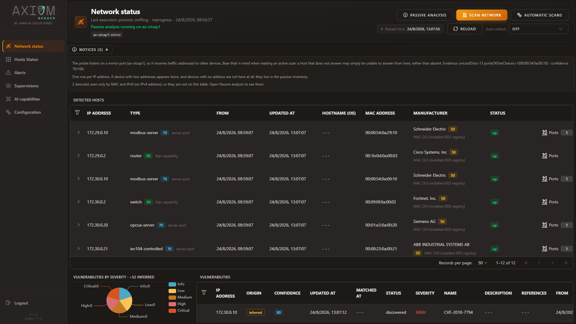
The console says so on the face of it. In the vulnerabilities table on Network status, every finding carries an Origin:

Origin	What it means
probe	The request was sent and the target answered. Demonstrated.
inferred	Derived from the device’s identity, with no traffic emitted. It is not proof — verify before acting.

An inferred finding also carries how complete the identity behind it was: the vendor only, the vendor and model, or the exact version. The probe never hands you a conclusion without telling you what it rests on.

Five things worth knowing

1. The passive probe decides whether an active scan means anything

The correct way to install a probe in an industrial network is on a mirror port or a TAP: it receives everything and cannot be answered. On such a port an active scan returns nothing — and that nothing means “nobody can reply to me from here”, not “there is nothing here”.

So classifying the connection point is the first thing the passive probe does, and the console leads with the verdict. Open Notices on Network status:

The probe listens on a mirror port, so it receives traffic addressed to other devices. Bear that in mind when reading an active scan: a host that does not answer may simply be unable to answer from here, rather than absent.

Without that line, half a day goes into working out why the discovery scan cannot find a network that is plainly there.

2. They discover along different axes

The passive probe indexes by MAC address. The active probes index by IP address. That is not a detail of bookkeeping — it changes what each one is capable of seeing at all.

• Passive analysis sees equipment with no IP address of its own: a fieldbus device, an unmanaged switch, a protection relay publishing multicast. None of these will ever produce a row in an active scan, however long you run it.
• Active scanning sees ports nobody happens to be using right now. A service that is listening but idle emits nothing to listen to, so passive analysis cannot know it is there.

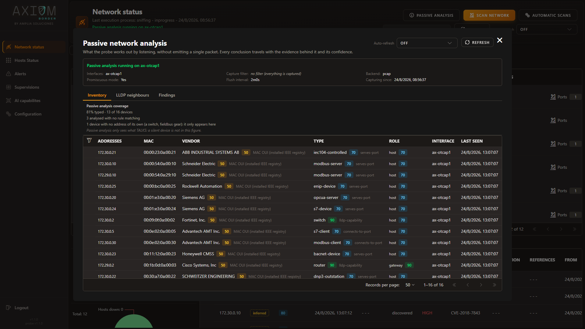
Neither set contains the other. In the capture below the passive inventory holds 16 devices where the address-indexed table on the same probe holds 12, and the coverage note explains the gap in the probe’s own words:

Note the closing caveat there, which is the honest limit of the technique: passive analysis only sees what talks — a silent device is not in this figure.

3. The passive probe feeds the active ones

The relationship is not merely parallel. What listening establishes is used to make the asking sharper:

• An SNMP target that is not yet in the inventory gets a quick discovery pass first, so the query goes to something known to be there.
• A vulnerability scan that comes back with nothing gets a discovery pass too, for one specific reason: to tell “unreachable” apart from “nothing wrong with it”. Those look identical in an empty report and mean completely different things.

4. Neither origin overwrites the other

Both write into the same identity record, and neither is allowed to win by arriving last. Each leaves its claim, its confidence and the evidence behind it, and the value you see is derived from all of them.

You can read this directly in the console. A manufacturer is shown with a confidence score and the source that produced it — the vendor registry installed on the probe, the device’s own declaration over its maker’s discovery protocol, or an active scan’s own table — each with its caveat attached. A registry entry names the network card; a device declaring itself names the device. Those are not the same claim, and the console does not pretend they are.

So when the active scan says Schneider Electric where the registry said Moxa, that disagreement is kept as data rather than resolved in silence. Nearly always it is telling you something true and useful: a network card from one vendor inside another vendor’s cabinet.

“Undecided” is a result, not a gap

A device the passive probe analysed without any rule matching is labelled undecided, and one written before passive analysis was available is labelled not analysed. They are shown differently on purpose: the first is a conclusion, the second is an absence of one. Neither is a failure, and neither is presented as an unknown you should chase.

5. An active scan does not close a passive inference

The one to hold on to.

A passive inference is not the outcome of a test. It is a statement about what a device is, drawn from how it behaves on the wire. An active scan failing to reproduce it does not refute it — the scan may not have looked for it, may not have been able to reach it, or may have been reading a mirror port where nothing can answer in the first place.

“I did not find it” is not “it is gone.” So a scan that comes back quiet leaves existing passive findings standing, and the console keeps showing them with their origin and their confidence. If you want one retracted, retract it deliberately — do not let an empty scan do it for you.

Side by side

	Active scanning	Passive analysis
Footprint on the network	Emits. Against a PLC, an aggressive scan is a genuine operational risk	Zero packets. Nothing a control device could misread
Identity is based on	The IP address	The MAC address, which survives a change of addressing
Equipment with no IP	Invisible	Inventoried
On a mirror port or TAP	No reply means no results	Works normally — and says why the active scan came back empty
Topology	Does not see it	Neighbours with their chassis and port, gateway verdict, address conflicts
Services	The real state of the port, confirmed	The services actually in use, and which side is serving
Traffic volume	—	Counters per host, and the breakdown behind them
Industrial posture	What the templates test for	What the equipment declares about itself as it operates

They are complementary, and the product treats them that way. Use the active probes to confirm; use the passive one to know what is worth confirming, and to see the part of the network the active ones cannot reach.

Next: From event to alarm — what happens once one of them finds something.

Three paths, one gate

Three different things can raise an alarm on an Axiom Border probe:

• A periodic check counting occurrences of an event over a window and finding too many.
• A dead-machine check finding a node that has gone silent — alarming on absence, which is the only way to catch a node that stopped reporting rather than one reporting something bad.
• A rule deciding, in code, that what it just saw is worth an alarm.

All three arrive at the same gate, and what that gate does is the single most operationally significant thing in this part of the product.

Coalescing by identity

Two alarms that say the same thing about the same device are the same alarm. When a condition trips repeatedly, the probe does not create a new alarm each time. It recognises the identity of the alarm — which agent, which device, which name and type, which severity, which underlying description — and folds the repeat into the alarm that is already open. What changes are its fields:

Field	Meaning
First seen	When the condition first held
Last seen	The most recent time it fired
Count	How many times it has fired

This pays twice over, and the two payoffs are worth separating because they matter to different people.

For the operator. A brute-force attempt that trips a threshold every five minutes for an hour is one thing happening, and it should read as one row with a count of twelve. Twelve identical rows are not twelve times the information — they are the same information, twelve times, pushing everything else off the screen. An alert repeated a thousand times is an alert, not a thousand alerts.

For the probe. Every distinct alarm is a distinct series in the history. Minting a fresh identity per occurrence makes that history grow without bound and slows every query made against it. Coalescing keeps the history of a busy probe queryable months later.

One row with a count is the signal, not a summary

When you see a count of 40 on an alarm, the probe is not telling you it collapsed 40 alarms to save room. It is telling you the condition has held 40 times since it first fired, and it is still open. The count is the severity information.

Acknowledging is not silencing

ACK on the Alerts view marks an alarm as seen, which closes the coalescing window on it.

The consequence is deliberate: the next occurrence after an acknowledgement opens a fresh alarm. It does not silently add one to a count on something you already dealt with. If the condition comes back, you get told again.

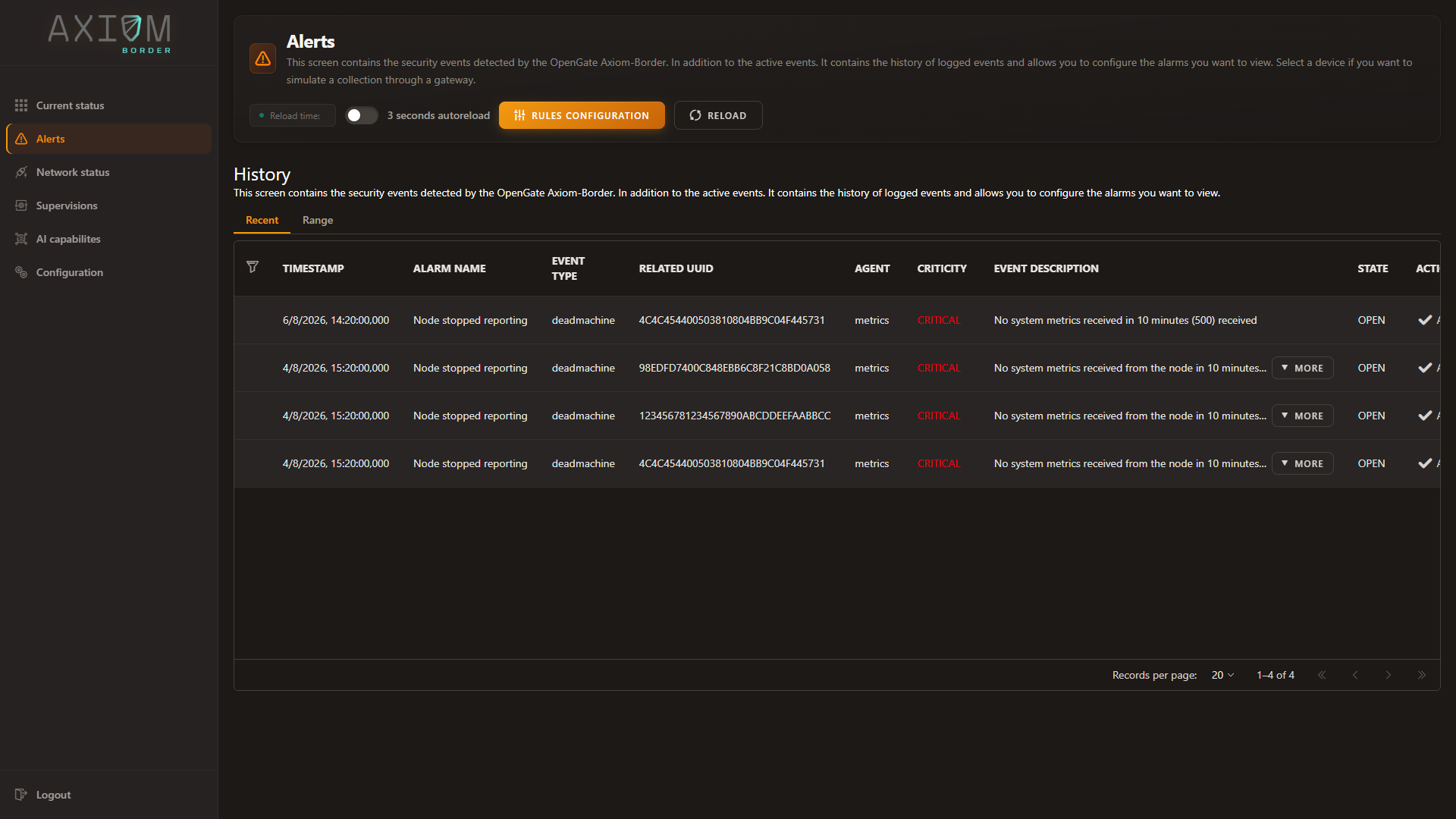
Two tabs sit above the table. Recent reads the probe’s live feed — the alarms it already holds in memory, answered instantly. Range queries a window of history instead, which is what you want when reconstructing an incident after the fact.

Open alarms survive a restart

The state of what is currently open is kept on the probe itself, not held in memory and lost on the next service restart. A probe that reboots comes back knowing which alarms were open and which had been acknowledged — and a quiet week does not make it forget either.

Rules that already know what changed

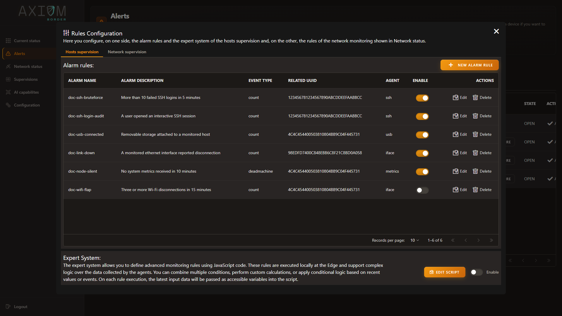
Rules are edited from Alerts → Rules configuration, where the declarative alarm rules sit in the upper table and the scripted Expert System sits below with its own enable switch:

There is one rule set per probe — one for discovery, one for vulnerability scanning, one for SNMP and one for passive analysis — and each receives that probe’s findings already enriched with what changed since the last time the probe saw the same thing:

• whether this is new,
• whether the value changed,
• and what the previous value was.

That is why a rule can say “this port is new” or “this value moved” without querying any history to find out. The comparison has already been made by the time the rule runs.

Each probe reports at its own granularity — one finding per vulnerability, one per host and one per port for discovery, one per value for SNMP, one per traffic flow and per port for passive analysis.

Rules are per probe, not across probes

A rule sees one probe’s findings. Correlating across probes — this port opened and that vulnerability appeared — is outside what the rules engine does; each evaluation belongs to a single probe. Build that correlation where you have the whole picture, in OpenGate.

The live feed

Every alarm is also pushed onto a small in-memory feed of the most recent events, oldest dropping off the end. It is what the console reads to paint its counter and its Recent tab, which is why those respond instantly however much history the probe has accumulated.

Full operating detail — creating checks, writing rules, the fields available to them — is in Alarms and rules.

Next: AI on the probe — when the rule needs a model to decide.

Inference happens on the node

Axiom Border can detect anomalies with machine-learning models, and the important word is where: the models run on the probe, in containers on the same machine. There is no call to an external service, no data sent away to be scored, and no dependency on a link being up.

That follows from the same premise as everything else here. A probe that had to reach a hosted model to decide would be a probe that stops deciding the moment the link drops — and would mean the traffic patterns of an isolated industrial network leaving it in order to be analysed.

The images the models run from are installed with the product, so an air-gapped probe can train and infer with nothing fetched from anywhere.

The circuit, end to end

flowchart LR
    D["Agent data<br>on the probe"] --> T["Trainer<br>container"]
    T --> M["Model<br>on the probe"]
    R["Rule"] -->|asks| M
    M -->|anomaly| R
    R --> A["Alarm"]

Training. The probe exports the data it holds for one agent and hands it to that agent’s trainer container. Retraining is scheduled rather than manual, can be cancelled while it runs, and its state is kept — so you can tell a model that is training from one that failed to.

Inference. The rule for an agent asks the model to score what it just received. If the answer comes back as an anomaly, the same rule raises the alarm.

And that alarm is an alarm like any other. It goes through the same coalescing gate described in From event to alarm — same identity rules, same count, same acknowledgement behaviour. An anomaly detected by a model is not a second class of signal with its own inbox; it lands on Alerts beside everything else, and an operator does not need to know which mechanism produced it to act on it.

Health. A rule can also read the model’s own metrics, and the probe polls the models’ health endpoints. This matters more than it sounds: a model that has stopped answering is then an observable fact rather than a silence that looks exactly like “no anomalies today”.

Where you manage it

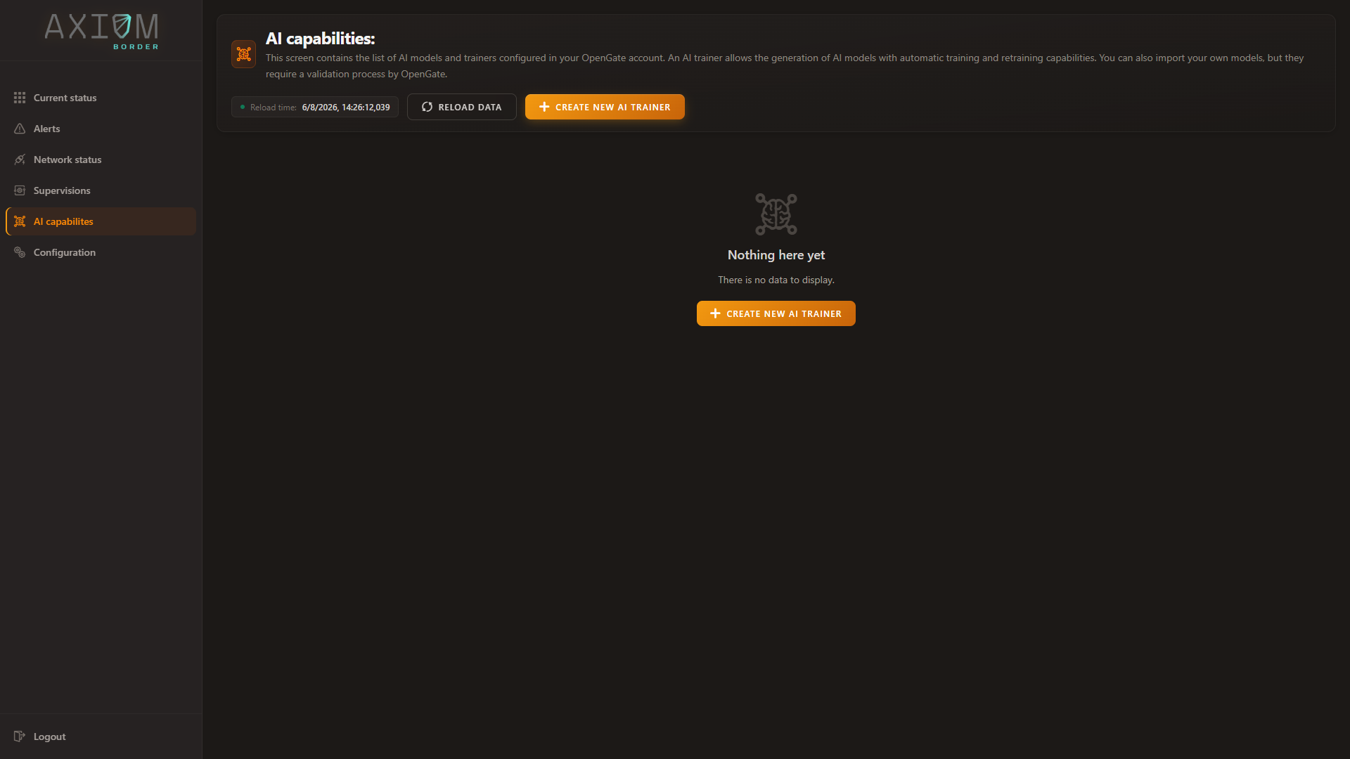
AI capabilities in the console lists the models and trainers configured on the probe:

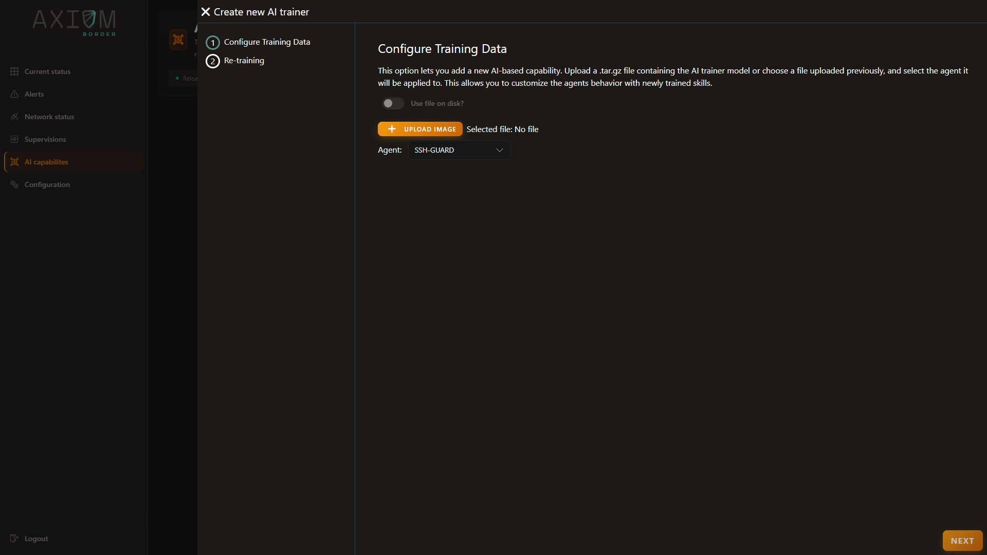
Adding one walks a wizard: upload the trainer package, or pick one already on the probe, and choose the agent it applies to.

Deploying, restarting, deleting and importing images are all driven from here. The rule that calls the model is enabled in step with the capability itself, so a model you deploy is a model that gets asked.

Linux, and the central role only

The container runtime the models need is Linux-only, and only the central role installs it. A monitoring node does not run models, and neither does a probe running natively on Windows — which is a development scenario, not a supported production one. On such a host the AI capability simply does not start, and the deployment controls have nothing behind them.

If you intend to use anomaly detection, deploy the probe as central on Linux.

Full operating detail — image formats, the training cycle, calling inference from a rule — is in AI capabilities.

Next: Security posture — the probe’s own attack surface, and where each kind of data lives.

The posture is deployed, not offered

Axiom Border sits inside the network it watches, which makes its own surface part of the product. What follows is not a list of hardening options to consider. It is what the installation puts in place, on both roles, with no decisions required from you.

Front	What is deployed
Console and API	HTTPS unconditionally, localhost included. There is no plaintext listener to fall back to
Certificate	Issued by a local authority on the probe at first boot — no external PKI, no internet. Replaceable with your own, and reloaded without dropping connections
Sessions	Token-based, signed with a key generated for that installation. Repeated failed logins from one address are throttled, and every login is written to the audit trail
Message bus	The embedded broker listens on loopback only, and its WebSocket listener is off. The console reaches it through a bridge inside the API’s own encrypted connection, using a single-use ticket that expires in seconds
Metrics ingestion	Not open to the network. The authentication step is waived only for callers inside a configured range, which defaults to loopback
Configuration	Reading the configuration back returns it with every secret redacted. Comments and formatting survive untouched
Cloud egress	Optional, and inert until configured. An insecure address stops the integration from starting at all

Why the certificate is self-issued

An air-gapped probe cannot reach a certificate authority, and requiring one before the console works would mean either no encryption or no probe. So the probe issues its own on first boot and is usable immediately over HTTPS.

Your browser will not recognise that authority, which is expected on first contact. If your organisation runs its own PKI, install its certificate on the probe instead — see Configuration.

The same applies to anything else that talks to the probe. Command-line examples throughout this documentation pass curl -sk, where -k is what accepts the probe’s own certificate; once you have installed a certificate your systems already trust, drop it.

Why an insecure cloud address is an error, not a warning

If you point the OpenGate integration at a plaintext address, the integration refuses to start. That is deliberate and it is not adjustable.

What travels over that link is the complete inventory of your network — every asset, every open port, every vulnerability found — together with the credential that authorises it. Sending that unencrypted is not a configuration preference with a trade-off. It is a mistake, and the probe treats it as one.

Secrets are never shown back to you

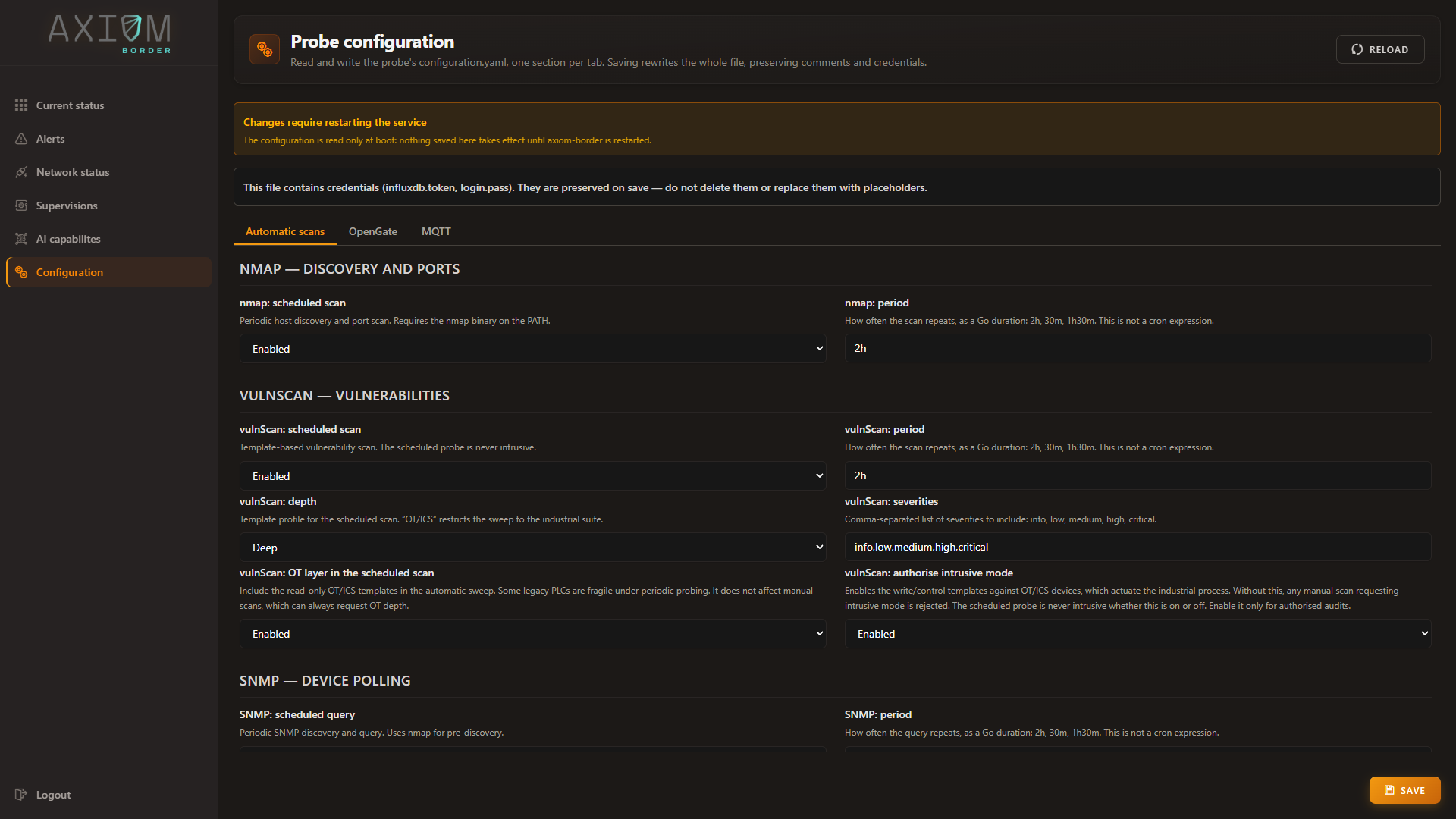
The Configuration view reads and writes the probe’s settings from the browser, and it says plainly what it does with credentials:

Each stored credential reads as redacted rather than as its value: leave it untouched to keep it, or type a new value over it to change it. Saving rewrites the file while preserving its comments — and a save that would quietly turn a protection off is rejected rather than accepted in silence.

Configuration is read at start-up

The banner at the top of that view is worth reading before you save: settings are read when the service starts, so nothing saved here takes effect until the probe restarts. The console offers to do it for you where the deployment allows.

Where each kind of data lives

Three stores, each chosen for what is asked of it:

Store	What it holds
The probe’s local state	Everything that must be exactly right and must survive a restart: alarm rules and scripts, device aliases, scan executions, SNMP credential profiles, the host and port inventory, findings, the provenance behind every identity claim, and the alarms currently open
The metrics database	Everything that is a series over time: agent metrics, the audit trail, network traffic, availability, scan metrics and alarm history
The in-memory feed	The most recent events per stream, so the console’s live counters answer instantly. Kept across restarts so a fresh probe comes back warm, and reconciled with the history in the background

The practical consequence for an operator: the console’s Recent tabs read the third one and are instant; the Range tabs read the second and are as fast as the window you ask for. Neither is more correct than the other — they are the same events, reached two ways.

What backing up means here

Because the three stores hold different things, a backup that covers only the metrics database keeps your history and loses your rules, profiles and inventory. Operation and maintenance covers what to back up and how to restore it.

That closes the tour. From here, Configuration is where you adapt a running probe to your environment.